The Gpx Time-Digitizing Correlator Data Viewer { Windows Menu }
The panel views shown in this document are from the
GViewer program running in Windows XP / Windows 2003.
Newer versions of Windows (7-10) render the panels
in modified color and form.

Complete functionality is maintained.
|
|

TG Graphing Window
         Clicking the 'TG Graphing Window' menu item opens the
      TG Graph:
         The TG Graph displays auto or cross correlation
      spectra with '0' time at the center and larger times
      extending toward the left and right edges.  This graph
      displays the data logarithmically in time with from
      1 to 14 overlapping data sets.  Each data set has a
      time range of two decades:

            1  -  100   100 ps bins       (FC data)
               or 100    50 ps bins       (FC data)
               or 100    33 ps bins       (FC data)
            2  -  100     1 ns bins       (Rebinned FC data)
            3  -  100    10 ns bins       (Rebinned FC data)
            4  -  100   100 ns bins       (Rebinned FC data)
            5  -  100     1 us bins       (BN data)
            6  -  100    10 us bins       (BN data)
            7  -  100   100 us bins       (BN data)
            8  -  100     1 ms bins       (BN data)
            9  -  100    10 ms bins       (BN data)
           10  -  100   100 ms bins       (BN data)
           11  -  100     1  s bins       (BN data)
           12  -  100    10  s bins       (BN data)
           13  -  100   100  s bins       (BN data)
           14  -  100  1000  s bins       (BN data)

         Each displayed data set has been normalized using
      only the acquisition time and count rates to produce
      the standard correlation display where a value of 1.0
      is the baseline.  The display baseline is at the top
      of the brown stripe in the display.  The alternate
      black and gray stripes are .1 intervals.  The maximum
      correlation value of 2.0 is at the top of the upper
      gray stripe.

         The horizontal scroll bar allows one to move the
      cross hairs (in the tan colored area around the spectra)
      to a particular time.  The channel number, counts in the
      channel, and the correlation time are displayed at the
      top of the spectra.  The vertical scroll bar may be used
      to change the vertical scaling.  The current vertical
      scaling factor is displayed above the spectra.


         The 'Graphing Control' tab associated with the displayed
      TG data is:
         The TG tab options include the ability to select
      the first displayed data set and the number of data sets
      to display.  The 'Average' option numerically averages
      the left / right spectra and displays the average on
      both the left and right sides of '0'.


         The 'Tweak Display' check box enables the normalization
      of the displayed FR spectra (.1, 1, 10, and 100ns binnings)
      to the BN spectra (1 microsecond and larger) by using a
      3 microsecond interval starting at the 9 microsecond point.
      The correlation method used for the FR spectra is
      sensitive to large variations in the count rate during
      acquisition.  This results in a very small decrease in the
      perceived count rate causing a small, usually less than
      a few tenths of a percent, mismatch between the FR and
      BN spectra.


         The 'Enable Draw Fit' check box in conjunction with the
      selection of a suitable equation and fitting parameters on
      the MrqFit -- Data Fitting window allows the display of a
      data fit superimposed upon the acquired data.
LG Graphing Window
         Clicking the 'LG Graphing Window' menu item opens the
      LG Graph:
         The LG Graph displays one of the correlation
      spectra with '0' time at the left.  This graph
      displays the data logarithmically in time with from
      1 to 14 overlapping data sets.  Each data set has a
      time range of two decades:

            1  -  100   100 ps bins       (FC data)
               or 100    50 ps bins       (FC data)
               or 100    33 ps bins       (FC data)
            2  -  100     1 ns bins       (Rebinned FC data)
            3  -  100    10 ns bins       (Rebinned FC data)
            4  -  100   100 ns bins       (Rebinned FC data)
            5  -  100     1 us bins       (BN data)
            6  -  100    10 us bins       (BN data)
            7  -  100   100 us bins       (BN data)
            8  -  100     1 ms bins       (BN data)
            9  -  100    10 ms bins       (BN data)
           10  -  100   100 ms bins       (BN data)
           11  -  100     1  s bins       (BN data)
           12  -  100    10  s bins       (BN data)
           13  -  100   100  s bins       (BN data)
           14  -  100  1000  s bins       (BN data)

         Each displayed data set has been normalized using
      only the acquisition time and count rates to produce
      the standard correlation display where a value of 1.0
      is the baseline.  The display baseline is at the top
      of the brown stripe in the display.  The alternate
      black and gray stripes are .1 intervals.  The maximum
      correlation value of 2.0 is at the top of the upper
      gray stripe.

         The horizontal scroll bar allows one to move the
      cross hairs (in the tan colored area around the spectra)
      to a particular time.  The channel number, counts in the
      channel, and the correlation time are displayed at the
      top of the spectra.

         The vertical scroll bar may be used to change the
      vertical scaling.  The current vertical scaling factor
      is displayed above the spectra.


         The 'Graphing Control' tab associated with the displayed
      LG data is:
         The LG tab options include the ability to select
      the first displayed data set and the number of data sets
      to display.


         The 'Tweak Display' check box enables the normalization
      of the displayed FR spectra (.1, 1, 10, and 100ns binnings)
      to the BN spectra (1 microsecond and larger) by using a
      3 microsecond interval starting at the 9 microsecond point.
      The correlation method used for the FR spectra is
      sensitive to large variations in the count rate during
      acquisition.  This results in a very small decrease in the
      perceived count rate causing a small, usually less than
      a few tenths of a percent, mismatch between the FR and
      BN spectra.


         The 'Enable Draw Fit' check box in conjunction with the
      selection of a suitable equation and fitting parameters on
      the MrqFit -- Data Fitting window allows the display of a
      data fit superimposed upon the acquired data.
FC Graphing Window
         Clicking the 'FC Graphing Window' menu item opens the
      FC Graph:
         The FC Graph displays a selected 'fast correlation'
      spectrum.  These spectra were created by the time-difference
      correlation process.  The valid time-difference range is
      131,072 bins at the 100 ps., 262,144 bins at 50 ps., or
      393,216 channels at 33 ps. resolution.

         The data is scaled so that the channel with the largest
      number of counts is displayed at full scale.

         The lower horizontal scroll bar allows one to move the
      cross hairs (in the tan colored area around the spectrum)
      to a particular time.  The channel number, counts in the
      channel, and the correlation time are displayed at the
      top of the spectrum.

         The vertical scroll bar may be used to change the
      vertical scaling.  The current vertical scaling factor
      is displayed above the spectrum.

         The upper horizontal scroll bar allows one to scroll
      the display through the complete data set using the range
      specified in the FC Graphing tab.  The beginning channel
      is displayed at the bottom of the spectrum.


         The 'Graphing Control' tab associated with the displayed
      FC data is:
         The FC tab options include the ability to select
      the time range of the displayed spectrum.
FR Graphing Window
         Clicking the 'FR Graphing Window' menu item opens the
      FR Graph:
         The FR Graph displays a selected rebinned
      'fast correlation' spectrum.  These spectra were
      created by rebinning the time-difference correlation
      data into 128 bins of 1, 10, or 100 ns.

         The data is scaled so that the channel with the largest
      number of counts is displayed at full scale.

         The horizontal scroll bar allows one to move the
      cross hairs (in the yellow colored area around the spectrum)
      to a particular time.  The channel number, counts in the
      channel, and the correlation time are displayed at the
      top of the spectrum.

         The vertical scroll bar may be used to change the
      vertical scaling.  The current vertical scaling factor
      is displayed above the spectrum.


         The 'Graphing Control' tab associated with the displayed
      FR data is:
         The FR tab options include the ability to select
      the time per bin of the displayed spectrum.
BN Graphing Window
         Clicking the 'BN Graphing Window' menu item opens the
      BN Graph:
         The BN Graph displays a selected correlation
      spectrum.  These spectra were created by the traditional
      processing of counts per bin data.  The binned data
      correlations were calculated for bin times of 1, 10, 100
      microseconds, 1, 10, 100 milliseconds, and 1, 10, 100,
      and 1000 seconds.

         The data is scaled so that the channel with the largest
      number of counts is displayed at full scale.

         The horizontal scroll bar allows one to move the
      cross hairs (in the yellow colored area around the spectrum)
      to a particular time.  The channel number, counts in the
      channel, and the correlation time are displayed at the
      top of the spectrum.

         The vertical scroll bar may be used to change the
      vertical scaling.  The current vertical scaling factor
      is displayed above the spectrum.


         The 'Graphing Control' tab associated with the displayed
      BN data is:
         The BN tab options include the ability to select
      the time per bin of the displayed spectrum.
Multiple TG Graphing Window
         Clicking the 'Multiple TG Graphing Window' menu item opens the
      Multiple TG Graph:
         The Multiple TG Graph displays multiple auto or
      cross correlation spectra with '0' time at the center and
      larger times extending toward the left and right edges.
      This graph displays the data logarithmically in time
      with from 1 to 14 overlapping data sets.  Each data
      set has a time range of two decades:

            1  -  100   100 ps bins       (FC data)
               or 100    50 ps bins       (FC data)
               or 100    33 ps bins       (FC data)
            2  -  100     1 ns bins       (Rebinned FC data)
            3  -  100    10 ns bins       (Rebinned FC data)
            4  -  100   100 ns bins       (Rebinned FC data)
            5  -  100     1 us bins       (BN data)
            6  -  100    10 us bins       (BN data)
            7  -  100   100 us bins       (BN data)
            8  -  100     1 ms bins       (BN data)
            9  -  100    10 ms bins       (BN data)
           10  -  100   100 ms bins       (BN data)
           11  -  100     1  s bins       (BN data)
           12  -  100    10  s bins       (BN data)
           13  -  100   100  s bins       (BN data)
           14  -  100  1000  s bins       (BN data)

         Each displayed data set has been normalized using
      only the acquisition time and count rates to produce
      the standard correlation display where a value of 1.0
      is the baseline.  The display baseline is at the top
      of the brown stripe in the display.  The alternate
      black and gray stripes are .1 intervals.  The maximum
      correlation value of 2.0 is at the top of the upper
      gray stripe.

         The horizontal scroll bar allows one to move the
      cross hairs (in the tan colored area around the spectra)
      to a particular time.  The channel number and the
      correlation time are displayed at the top of the spectra.

         The vertical scroll bar may be used to change the
      vertical scaling.  The current vertical scaling factor
      is displayed above the spectra.


         The 'Graphing Control' tab associated with the displayed
      Multiple TG data is:

         The Multiple TG tab options include the ability to
      select the first displayed data set and the number of
      data sets to display.


         The 'Tweak Display' check box enables the normalization
      of the displayed FR spectra (.1, 1, 10, and 100ns binnings)
      to the BN spectra (1 microsecond and larger) by using a
      3 microsecond interval starting at the 9 microsecond point.
      The correlation method used for the FR spectra is
      sensitive to large variations in the count rate during
      acquisition.  This results in a very small decrease in the
      perceived count rate causing a small, usually less than
      a few tenths of a percent, mismatch between the FR and
      BN spectra.


         The 'Enable Draw Fit' check box in conjunction with the
      selection of a suitable equation and fitting parameters on
      the MrqFit -- Data Fitting window allows the display of a
      data fit superimposed upon the acquired data.
Multiple LG Graphing Window
         Clicking the 'Multiple LG Graphing Window' menu item opens the
      Multiple LG Graph:
         The Multiple LG Graph displays multiple auto or
      cross correlation spectra with '0' time at the left.
      This graph displays the data logarithmically in time
      with from 1 to 14 overlapping data sets.  Each data
      set has a time range of two decades:

            1  -  100   100 ps bins       (FC data)
               or 100    50 ps bins       (FC data)
               or 100    33 ps bins       (FC data)
            2  -  100     1 ns bins       (Rebinned FC data)
            3  -  100    10 ns bins       (Rebinned FC data)
            4  -  100   100 ns bins       (Rebinned FC data)
            5  -  100     1 us bins       (BN data)
            6  -  100    10 us bins       (BN data)
            7  -  100   100 us bins       (BN data)
            8  -  100     1 ms bins       (BN data)
            9  -  100    10 ms bins       (BN data)
           10  -  100   100 ms bins       (BN data)
           11  -  100     1  s bins       (BN data)
           12  -  100    10  s bins       (BN data)
           13  -  100   100  s bins       (BN data)
           14  -  100  1000  s bins       (BN data)

         Each displayed data set has been normalized using
      only the acquisition time and count rates to produce
      the standard correlation display where a value of 1.0
      is the baseline.  The display baseline is at the top
      of the brown stripe in the display.  The alternate
      black and gray stripes are .1 intervals.  The maximum
      correlation value of 2.0 is at the top of the upper
      gray stripe.

         The horizontal scroll bar allows one to move the
      cross hairs (in the tan colored area around the spectra)
      to a particular time.  The channel number and the
      correlation time are displayed at the top of the spectra.

         The vertical scroll bar may be used to change the
      vertical scaling.  The current vertical scaling factor
      is displayed above the spectra.


         The 'Graphing Control' tab associated with the displayed
      Multiple LG data is:
         The Multiple LG tab options include the ability to
      select the first displayed data set and the number of
      data sets to display.


         The 'Tweak Display' check box enables the normalization
      of the displayed FR spectra (.1, 1, 10, and 100ns binnings)
      to the BN spectra (1 microsecond and larger) by using a
      3 microsecond interval starting at the 9 microsecond point.
      The correlation method used for the FR spectra is
      sensitive to large variations in the count rate during
      acquisition.  This results in a very small decrease in the
      perceived count rate causing a small, usually less than
      a few tenths of a percent, mismatch between the FR and
      BN spectra.


         The 'Enable Draw Fit' check box in conjunction with the
      selection of a suitable equation and fitting parameters on
      the MrqFit -- Data Fitting window allows the display of a
      data fit superimposed upon the acquired data.
Combined TG Graphing Window
         Clicking the 'Combined TG Graphing Window' menu item opens the
      Combined TG Graph:
         The Combined TG Graph displayss multiple auto or cross
      correlation spectra with '0' time at the center and and larger
      times extending toward the left and right edges into a single
      graph.  This graph displays the data logarithmically in time
      with from 1 to 14 overlapping data sets.  Each data
      set has a time range of two decades:

            1  -  100   100 ps bins       (FC data)
               or 100    50 ps bins       (FC data)
               or 100    33 ps bins       (FC data)
            2  -  100     1 ns bins       (Rebinned FC data)
            3  -  100    10 ns bins       (Rebinned FC data)
            4  -  100   100 ns bins       (Rebinned FC data)
            5  -  100     1 us bins       (BN data)
            6  -  100    10 us bins       (BN data)
            7  -  100   100 us bins       (BN data)
            8  -  100     1 ms bins       (BN data)
            9  -  100    10 ms bins       (BN data)
           10  -  100   100 ms bins       (BN data)
           11  -  100     1  s bins       (BN data)
           12  -  100    10  s bins       (BN data)
           13  -  100   100  s bins       (BN data)
           14  -  100  1000  s bins       (BN data)

         Each displayed data set has been normalized using
      only the acquisition time and count rates to produce
      the standard correlation display where a value of 1.0
      is the baseline.  The display baseline is at the top
      of the brown stripe in the display.  The alternate
      black and gray stripes are .1 intervals.  The maximum
      correlation value of 2.0 is at the top of the upper
      gray stripe.

         The horizontal scroll bar allows one to move the
      cross hairs (in the tan colored area around the spectra)
      to a particular time.  The channel number and the
      correlation time are displayed at the top of the spectra.

         The vertical scroll bar may be used to change the
      vertical scaling.  The current vertical scaling factor
      is displayed above the spectra.


         The 'Graphing Control' tab associated with the displayed
      Combined TG data is:
         The Combined TG tab options include the ability to
      select the first displayed data set and the number of
      data sets to display.


         The 'Tweak Display' check box enables the normalization
      of the displayed FR spectra (.1, 1, 10, and 100ns binnings)
      to the BN spectra (1 microsecond and larger) by using a
      3 microsecond interval starting at the 9 microsecond point.
      The correlation method used for the FR spectra is
      sensitive to large variations in the count rate during
      acquisition.  This results in a very small decrease in the
      perceived count rate causing a small, usually less than
      a few tenths of a percent, mismatch between the FR and
      BN spectra.


         The 'Enable Draw Fit' check box in conjunction with the
      selection of a suitable equation and fitting parameters on
      the MrqFit -- Data Fitting window allows the display of a
      data fit superimposed upon the acquired data.
Combined LG Graphing Window
         Clicking the 'Combined LG Graphing Window' menu item opens the
      Combined LG Graph:
         The Combined LG Graph displays multiple auto or cross
      correlation spectra with '0' time at the left in a single
      graph.  This graph displays the data logarithmically in time
      with from 1 to 14 overlapping data sets.  Each data set
      has a time range of two decades:

            1  -  100   100 ps bins       (FC data)
               or 100    50 ps bins       (FC data)
               or 100    33 ps bins       (FC data)
            2  -  100     1 ns bins       (Rebinned FC data)
            3  -  100    10 ns bins       (Rebinned FC data)
            4  -  100   100 ns bins       (Rebinned FC data)
            5  -  100     1 us bins       (BN data)
            6  -  100    10 us bins       (BN data)
            7  -  100   100 us bins       (BN data)
            8  -  100     1 ms bins       (BN data)
            9  -  100    10 ms bins       (BN data)
           10  -  100   100 ms bins       (BN data)
           11  -  100     1  s bins       (BN data)
           12  -  100    10  s bins       (BN data)
           13  -  100   100  s bins       (BN data)
           14  -  100  1000  s bins       (BN data)

         Each displayed data set has been normalized using
      only the acquisition time and count rates to produce
      the standard correlation display where a value of 1.0
      is the baseline.  The display baseline is at the top
      of the brown stripe in the display.  The alternate
      black and gray stripes are .1 intervals.  The maximum
      correlation value of 2.0 is at the top of the upper
      gray stripe.

         The horizontal scroll bar allows one to move the
      cross hairs (in the tan colored area around the spectra)
      to a particular time.  The channel number and the
      correlation time are displayed at the top of the spectra.

         The vertical scroll bar may be used to change the
      vertical scaling.  The current vertical scaling factor
      is displayed above the spectra.


         The 'Graphing Control' tab associated with the displayed
      Combined LG data is:
         The Combined LG tab options include the ability to
      select the first displayed data set and the number of
      data sets to display.


         The 'Tweak Display' check box enables the normalization
      of the displayed FR spectra (.1, 1, 10, and 100ns binnings)
      to the BN spectra (1 microsecond and larger) by using a
      3 microsecond interval starting at the 9 microsecond point.
      The correlation method used for the FR spectra is
      sensitive to large variations in the count rate during
      acquisition.  This results in a very small decrease in the
      perceived count rate causing a small, usually less than
      a few tenths of a percent, mismatch between the FR and
      BN spectra.


         The 'Enable Draw Fit' check box in conjunction with the
      selection of a suitable equation and fitting parameters on
      the MrqFit -- Data Fitting window allows the display of a
      data fit superimposed upon the acquired data.
DA Graphing Window
         Clicking the 'DA Graphing Window' menu item opens the
      DA Graph.

         The DA graphing window is strictly a diagnostic
      tool used to study the systematics of the TDC-GPX
      time-digitizing chip.  The TDC-GPX can be programmed
      for three resolutions, 100, 50, or 33 picoseconds.  The
      bin times are determined by the propagation of a clock
      signal through multiple logic elements.  The total
      time through some N elements is controlled by an
      applied voltage to exactly match some external frequency
      source (a precision quartz crystal oscillator).  The
      locking to the external frequency source (and its phase)
      is controlled by an external circuit called a PLL (Phase
      Locked Loop).

         The manufacture's data sheet explicitly states that
      there is a strong DNL (Differential Non-Linearity)
      between adjacent bins.  A DA graph with data taken
      at a 100 picosecond resolution shows the effect.
         The DA Graph displays a summed spectrum
      where the range is 216 bins.  This was selected to
      be 4 times the observed TDC-GPX DNL period of 54 bins.
      The [296] signifies that 296 segments of 216 bins,
      corresponding to the full scale time-digitizing range
      of 63,936 intervals for the Gpx Time-Digitizer
      Instrument, are summed to provide the spectrum.
      The average differential non-linearity is about 10%
      between adjacent pairs.

         The data is scaled so that the channel with the largest
      number of counts is displayed at full scale.

         The horizontal scroll bar allows one to move the
      cross hairs (in the pink colored area around the spectrum)
      to a particular time.  The channel number, counts in the
      channel, and the channel time are displayed at the
      top of the spectrum.

         The vertical scroll bar may be used to change the
      vertical scaling.  The current vertical scaling factor
      is displayed above the spectrum.

         The average and root-mean-square (RMS) scatter of
      data is calculated as an indication of the systematic
      error.

         The Correction Averages indicate the average of the
      fraction of events that are moved up / down to affect
      a correction for the Differential Non-Linearity.


         The 'Graphing Control' tab associated with the displayed
      DA data is:

         The DA tab also displays a distribution of the
      counts in the time bins where the far left is the lowest
      counts in a bin and the far right having the largest
      counts in a bin.  One notes that the distribution of
      counts per bin is centered around two dominant times.


         The DA graph for the 33 picosecond resolution
      is very different:
         This DA Graph shows a DNL where it is difficult to
      discern its characteristic time.  However it has been
      determined to have a DNL period of 3 times the base
      DNL period of 54 bins.  The DA graph thus was chosen
      to have 4 * the DNL period, 648 bins. The [98]
      signifies that 98 segments of 648 bins were used to
      create the display.


         The DNL algorithm is implemented by summing the raw
      TDC-GPX time-digitizer channel data modulus 216, 432, or
      648 for 100, 50, or 33 ps. respectively into a DNL array
      of 216, 432, or 648 elements.  At acquisition startup the
      DNL calculational threshold is set at 32 counts per bin.
      When the threshold value is reached an array of transfer
      coefficients is calculated for each DNL array element.
      Each coefficient specifies the fraction of the events in
      the corresponding DNL array element which must be bumped
      into an adjacent DNL array element to remove the
      Differential Non-Linearity.  These coefficients are then
      used to bump a fraction of the acquired data (modulo 216,
      432, or 648) into adjacent time bins.  After the transfer
      coefficents are calculated the calculational threshold
      is increased by a factor of two upto a maximum of 32768
      counts per bin.  From that point on the number of events
      in each DNL array element is divided by two after the
      coefficient calculation.  Additionally to reduce any
      systematic errors due to the bumping direction the
      bumping direction is reversed after every coefficient
      calculation.  This process continues during the
      acquisition cycle allowing the corrections to
      dynamically change as required.

         Each TDC-GPX time-digitizing channel used for data
      acquisition has its own independent DNL correction
      array.  TDC-GPX time-digitizing channels used for time
      markers are not corrected for DNL.


         The 'Graphing Control' tab associated with the displayed
      DA data is:

         The distribution of counts per bin is spread over
      a range of times and not localized around a dominant time.


         Note the 'DNL Processing Select' option on the DA
      graphing control tab.  The DA graphs shown so far
      are 'Pre' spectra, those with no DNL corrections applied.
      The following graphs are for the 'Post' spectra and
      have the DNL corrections applied.

      First, the 100 picosecond resolution data:

         The 'Post' spectra with DNL corrections has removed
      the predominate alternate channel differences.


         The 'Graphing Control' tab associated with the displayed
      DA data is:
         The 'Post' distribution with DNL corrections shows
      the central single distribution of counts per channel.


      Second, the 33 picosecond resolution data:

         The 'Post' spectra with DNL corrections has removed
      the major non-linearity.  The average and RMS scatter has
      been reduce by a factor of 4.


         The 'Graphing Control' tab associated with the displayed
      DA data is:

         The 'Post' distribution with DNL corrections shows
      the very strongly centralized single distribution of
      counts per channel.
DG Graphing Window
         Clicking the 'DG Graphing Window' menu item opens the
      DG Graph.

         The DG graphing window is a diagnostic tool used
      to observe the effects of the various corrections
      on the data from the TDC-GPX time-digitizing chip.
      The 'Pre' and 'Post' correction display options
      are available.  The DG/DA processing software is
      configured to have a basic timing conversion interval
      of 63,936 bins independent of resolution.


      DG (Pre) graph with 100 picosecond resolution data:
         The data is scaled so that the channel with the largest
      number of counts is displayed at full scale.

         The lower horizontal scroll bar allows one to move the
      cross hairs (in the pink colored area around the spectrum)
      to a particular bin.  The channel number, counts in the
      channel, and the bin time are displayed at the top of
      the spectrum.

         The vertical scroll bar may be used to change the
      vertical scaling.  The current vertical scaling factor
      is displayed above the spectrum.

         When the upper horizontal scroll bar is shown one can
      scroll the display through the complete data set using
      the range specified in the DG Graphing tab.  The beginning
      channel is displayed at the bottom of the spectrum.


         The 'Graphing Control' tab associated with the displayed
      DG data is:

         The DG tab options include the ability to select
      the time range of the displayed spectrum.


         The DG (Pre) graph for the 33 picosecond resolution
      is quite similar:
         The 'Graphing Control' tab associated with the displayed
      DG data is:
         The distribution of counts per bin is spread over
      a range indicating it is not statistical in nature.


         Note the 'DNL Processing Select' option on the DG
      graphing control tab.  The DG graphs shown so far
      are 'Pre' spectra, those with no DNL corrections applied.
      The following graphs are for the 'Post' spectra and
      have the DNL corrections applied.

      The DG (Post) graph for 100 picosecond resolution data:
         The 'Graphing Control' tab associated with the displayed
      DG data is:

         The distribution of counts per bin is now more
      statistical as shown by its gaussian shape.


      The DG(Post) graph for 33 picosecond resolution data:
         The 'Graphing Control' tab associated with the displayed
      DG data is:
RB Graphing Window
         Clicking the 'RB Graphing Window' menu item opens
      the RB Graph:
         The RB graphing window displays a sequence of rebinned
      fast correlation data (FC) which has 131,072 channels,
      262,144 channels, or 393,216 channels at resolutions of
      100 ps., 50 ps., or 33 ps. respectively.


         The 'Graphing Control' tab associated with the displayed
      RB data is:
         The RB tab options include the ability to select
      the correlation spectrum type to be rebinned and the
      graphing mode for the displayed data.


         The fast correlation data can be rebinned by specifying
      the rebinning parameters on the 'Data Binning' tab:
         The data rebinning is controlled by the 20 parameter
      sets on the four group tabs.  The three parameters are
      (1) the beginning channel, (2) the ending channel, and
      (3) the number of channels to average per displayed point.
      To configure a parameter set clear the checkbox on the right,
      enter the three parameters, and then set the checkbox to
      enable the parameter set.  When the checkbox is set the
      entered parameters will be checked to verify correct
      boundary conditions and updated if required.  The data
      associated with the checked parameter set will then be
      displayed along with all other checked parameter sets.


         The 'Mode/Range' tab controls how the parameter sets
      are interpreted and the range of the data to be displayed:
         The display mode is selected as channels or nanoseconds.
      The display range can be selected from the 4 fixed settings
      or a user specified range can be specified and selected.

         After specifying and adjusting the parameter sets to
      display the data in the form required the data can be exported
      to a data file by selecting the 'Create XY Data' item on
      the Viewers' main menu:
         The output file will be a text file having four
      parameters per line corresponding to the X position in time,
      the Y amplitude as a normalized correlation spectra with a
      range of 0-2 with a baseline of 1, the statistical error
      of the normalized correlation spectrum, and the Y amplitude
      of any fit function selection.  If a fit was not performed
      then the output for this parameter will be 0.  The output
      data will contain all of the rebinned data plus all other
      binned data, FR and BN spectra, in sequential order excluding
      lower resolution overlapping data.  The exported data
      file can be easily imported into an external analysis
      or viewing program.
RT Graphing Window
         Clicking the 'RT Graphing Window' menu item opens
      the RT Graph:
         The RT graphing window can be configured to
      show any of the 12 acquisition channels simultaneously.
      The count rates for any 2 acquisition channels may be
      displayed using the drop-down selection boxs.

         The horizontal scroll bar allows one to move the
      cross hairs (in the yellow colored area around the spectrum)
      to a particular time.  The channel time and channel
      count rates are shown.
Overlay Control Window
        Clicking the 'Overlay Control Window' menu item
      opens the 'Overlay Control' window:
The Overlay Control window allows upto 10 data sets to
be loaded and displayed as overlays. Clicking on any
of the 10 selection buttons will open a file selection
dialog box:
 Select a file and click 'Open' to load the data or
select 'Cancel' to abort the file selection. After
loading the data the Overlay Control window will
show the data file name and automatically set the
'Enable' check box.
Select a file and click 'Open' to load the data or
select 'Cancel' to abort the file selection. After
loading the data the Overlay Control window will
show the data file name and automatically set the
'Enable' check box.
 To remove a data file entry double click on the data
file name. A message will appear asking for confirmation
that the data set should be removed.
To remove a data file entry double click on the data
file name. A message will appear asking for confirmation
that the data set should be removed.
 Clicking 'Yes' will remove the data set and clear the
'Enable' check box if set.
After data has been loaded into the overlay data
arrays the data may be displayed with a spectrum
by selecting the 'Enable Overlay' check box on an
overlay supported Graphing Control Tab.
The following shows a non overlayed 'Combined TG'
display followed by an overlayed display:
Clicking 'Yes' will remove the data set and clear the
'Enable' check box if set.
After data has been loaded into the overlay data
arrays the data may be displayed with a spectrum
by selecting the 'Enable Overlay' check box on an
overlay supported Graphing Control Tab.
The following shows a non overlayed 'Combined TG'
display followed by an overlayed display:
The triplets of color following each data set specify
the colors displayed for that data set. The three colors
are used by the multisegment spectrum displays (CL, CT,
LG, ML, MT, and TG) while the first color of the triplet
is used for the single segment displays (BN, DA, DG, FC,
and FR).
The colors of overlay [1] are fixed, however the colors
for overlays [2] through [10] may be changed. Double click
a color to bring up the basic color selection box:
 To create a custom color click 'Define Custom Colors >>'.
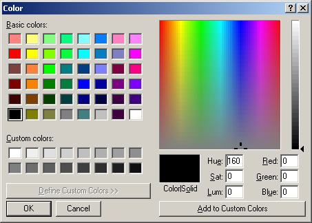 Use the '?' button for more information.
To restore the color triplets to their default values click the
task bar 'Colors' option and click 'Restore Default Color Scheme'.
Use the '?' button for more information.
To restore the color triplets to their default values click the
task bar 'Colors' option and click 'Restore Default Color Scheme'.
 To save the overlay configuration at program exit and
restore the configuration at the next program startup
click 'Files' then 'Save/Restore Overlay File Entries'.
Click 'Files' to verify that 'Save/Restore ...' is checked.
To save the overlay configuration at program exit and
restore the configuration at the next program startup
click 'Files' then 'Save/Restore Overlay File Entries'.
Click 'Files' to verify that 'Save/Restore ...' is checked.
 To discard the overlay configuration at program exit
click 'Files' then 'Save/Restore Overlay File Entries'.
Click 'Files' to verify that 'Save/Restore ...' is unchecked.
To discard the overlay configuration at program exit
click 'Files' then 'Save/Restore Overlay File Entries'.
Click 'Files' to verify that 'Save/Restore ...' is unchecked.
        Clicking 'Help' on the 'Overlay Control' window brings up a
      help window having a summary of the options described above.
MRQ Data Fitting
        Clicking the 'MrqFit Data Fitting' menu item opens
      the MrqFit Data Fitting Window.  The 'MrqFit Data Fitting' window
      is the control center for configuring the parameters required to
      perform data fitting and graphing of the fitting results.
      Tab 1:  Fitting Configuration


         The 'Fitting Configuration' tab contains the following selections:

         a) Correlation Fitting Configuration Selection

            Automatic configuration selection is the default mode for
            specifying the binnings and correlation selection.  The
            selection is made by

               1) Select one of the LG, TG, Multiple LG, or Multiple TG
                  spectra for display.

               2) Check the selected 'Enable Draw Fit' box.

            A manual selection option is available for specifying the
            fitting selection for special circumstances.

            The selections are LG, TG, Multiple LG, and Multiple TG.  The
            data fitting is performed using the spectrum selections from
            these graphing windows.  The specific detector(s) selected for
            display are not relevant to this configuration.


            Data Select(First Binning, Binnings) and
            Correlation Select(AC or CC) from each detector pair


            Data Select(First Binning, Binnings),
            Correlation Select(AC or CC) from each detector pair, and
            Graphing Mode(Average) from each detector pair


            Data Select(First Binning, Binnings) and
            Correlation Select(AC or CC)


            Data Select(First Binning, Binnings),
            Correlation Select(AC or CC), and
            Graphing Mode(Average)


            Data Select(First Binning, Binnings) and
            Correlation Select(AC or CC)


            Data Select(First Binning, Binnings),
            Correlation Select(AC or CC), and
            Graphing Mode(Average)


         b) Spectral Fitting Parameters

            All the spectra to fit set in Tab 5 are processed.

            Maximum Number of Fitting Iterations for each Spectra [1, 2, 5, 10, 25, 50]
            specifies the maximum number of fitting iterations to perform on
            a single spectrum at each 'fit' update.  The iterations will
            terminate if the fractional change limit in Chi^2 occurs.


         c) Fitting Points

            Select Data Points to Fit:

              1) All Data Points - Fitting function uses all
                 the data points selected by LG, TG, Multiple LG,
                 or Multiple TG options.

              2) Log Spaced Points - Fitting function uses data
                 rebinned into 10 points per decade of time such
                 that the points are equally spaced on a logarithmic
                 time scale.  The data points are rebinned from all
                 the data points selected by LG, TG, Multiple LG,
                 or Multiple TG options.


         d) Fitting Weight

            Select how the fitting function weights the data points:

              1) Statistical - The fitting function adjusts the
                 relative significance of the data point based on
                 the statistical error of the data.  Data with
                 smaller statistical errors have more significance.

              2) Equal - The fitting function treats every data
                 point with equal significance.  Statistical
                 errors are not used.


         e) Fractional Change in Chi^2 to Terminate Fit

            This parameter specifies the lower limit of the absolute fractional change
            in the normalized Chi^2 value to terminate the fitting iterations.  The
            selections are [.01, .001, .0001, .00001, .000001].  The default is .0001.


         The two comand buttons:

            'Restart All Fitting' resets the fitting functions to their initial
            values and prepares for a new fitting sequence.

            'Run Fitting Sequence' initiates a fitting sequence.
      Tab 2:  Fitting Function Selection


         The loaded data is processed using the Levenberg-Marquardt
      method attempting to reduce the value Chi^2 of a fit between a
      set of data points x[1..ndata], y[1..ndata] with individual
      standard deviations sig[1..ndata], and a nonlinear function
      dependent on n coefficients a[1..n].  The algorithm allows
      selected initial parameter values to be held constant during
      the fitting process.


        The 'All Channels' 'Restart' button resets the fitting functions
      for all channels (1-12) to their initial values and prepares for
      a new fitting sequence.  The 'All Channels' 'Fit' button initiates
      a fitting sequence for all active channels (1-12).


         The 'Fitting Function Selection' tab allows the selection of a
      fitting equation for each of the 12 detectors.  The equation is
      selected from the dropdown box:


      The equations and corresponding displays are:

      1) Single Exponential                                          [3 independent terms]


      2) Single Stretched Exponential                                [4 independent terms]


      3) Double Exponential                                          [6 independent terms]


      4) Double Stretched Exponential                                [8 independent terms]


      5) Double Exponential with Oscillatory Term                    [7 independent terms]


      6) Triple Exponential                                          [8 independent terms]


      7) Special Function                                          [11 independent terms]


      8) Special Function                                          [10 independent terms]


         Clicking 'Equation Details' on the task bar opens the
      MrqFit Equations Details Window:


      Selecting the appropriate equation tab gives the equation
      details and computation partial derivatives required by the
      Levenberg-Marquardt fitting method.


         The features of the fitting function display are described
      in detail for each row of elements:


         The Chi^2 panel displays the normalized Chi Square value
      followed by the number of fit iterations before the fitting
      was terminated by the Chi^2 limit or iteration limit.

         Pressing the RED Restart button initializes the fitting
      process for this detector by clearing the current fit
      values and loading the initial parameter values for the
      fitting function.

         Pressing the GREEN Fit button initiates a fitting
      sequence for this detector.  The number of iterations
      is determined by the values selected in the Maximum
      Number of Fitting Iterations on Tab 1.


         Each independent fitting parameter has an associated
      button which specifies if this parameter is a variable
      or fixed value.  A Light-Green button indicates a varible
      parameter and a Light-Red button indicates a fixed value.
      Pressing a button toggles the parameter from variable to
      fixed or fixed to variable.  Changes to the parameter
      type become effective when the RED Restart button is
      pressed or the 'Restart All Fitting' button is pressed
      on Tab 1.


         The initial fitting function parameter values are
      shown with a Light-Green background for variable parameters
      and Light-Red for fixed parameters.  New values for these
      parameters may be entered into the boxes, if an invalid
      value is entered the original value is restored.  Changes
      to the parameter values become effective when the RED
      All Channels 'Restart' button, RED 'Restart' button, or the
      'Restart All Fitting' button is pressed on Tab 1.


         The resulting fit values are displayed as GREEN for
      variables and RED for fixed parameters.

         An initial fitting function parameter value may be
      loaded from the result fit value by 'double-clicking'
      the result fit value.


      Note:
         If the fitting function selection is changed the new
      fitting function initial parameters will be displayed.
      However, the previous fitting function is still active
      and the displayed fit values will continue to be updated.
      This condition is indicated by the Light-Yellow background
      for displayed fitting results.  Changes to the fitting
      function become effective when the RED 'Restart' button,
      RED All Channels 'Restart' button, or the 'Restart All Fitting'
      button is pressed on Tab 1.


         The 'MrqFit Data Fitting' File Menu:


      gives the option to save the fit values to a file.
      A standard Save As file dialog box will open:
      Tab 3:  Scattering Configuration


         The scattering configuration tab is used to specify the
      scattering parameters and configuration.  These parameters
      will then be used to calculate the 'q' values of the scattered
      photons.  The parameters and configuration items are:

      1) Detector scattering angles in degrees
      2) Laser light incident angle in degrees
      3) Laser light wavelength in microns
      4) Parallel index of refraction
      5) Perpendicular index of refraction
      6) Incident Polarization ( [H]orizontal or [V]ertical )
      7) Scattering Polarization ( [H]orizontal or [V]ertical )
      8) Sample Type Selection:
         a) q
            1) Isotropic
            2) LC - Liquid Crystal    Homeotropic
            3) LC - Liquid Crystal    Planar [H]orizontal
         b) q - parallel
            1) LC - Liquid Crystal    Homeotropic
            2) LC - Liquid Crystal    Planar [H]orizontal
         c) q - perpendicular
            1) LC - Liquid Crystal    Homeotropic
            2) LC - Liquid Crystal    Planar [H]orizontal
            2) LC - Liquid Crystal    Planar [V]ertical

      The square of the 'Q Selection' values may then be used as the
      Y-Axis scaling of the 'Parameter Graph' displayed in Tab 6.
      Tab 4:  Q Calculations


         The Q Caculation Tab simply shows the calculated values for
      q, q-parallel, and q-perpendicular for each detector scattering
      angle based upon the parameter values and q selection in Tab 3.
      Tab 5:  Fit Parameters to Graph


         The 'Fit Parameters to Graph' tab enables fitting of selected
      detector data (C1 - C12) and the graphing of selected parameters
      during data acquisition.

         The detector (C1-C12) check box(s) must be checked to enable
      data fitting for a specific detector.  A detector's parameter
      check box(s) must be checked to enable graphing of the parameter
      in the 'Fit Parameter Graph' in Tab 6.

      Note:
         The parameter check box selections for detector (C1-C12) are
         associated with the currently selected fitting function.
         Changing the fitting function for a detector will change the
         parameter check box selections.

      Note:
         Graphing windows LG, TG, ML (Multiple LG), and MT (Multiple TG)
         DO NOT require a detector check box to be checked.  The
         'Enable Draw Fit' check boxs on the LG, TG, ML, and MT 'Graphing
         Control Window' tabs independently enable fitting for the spectra
         specified in the Graphing Control Window.
      Tab 6:  Fit Parameter Graphing


         The 'Fit Parameter Graphing' tab simply displays the selected
      parameters from the data fitting.  The parameter data is color
      coded as noted.


         The X-Axis drop down selection box


      selects the X-Axis scaling as one of the following:

      1) Cn
      2) Angle
      3) (Q Selection)^2

      where the square of the 'Q Selection' value is from
      the 'Scattering Configuration' of Tab 3.


         The Y-Axis drop down selection box


      selects the Y-Axis scaling as one of the following:

      1) Linear
      2) Log
      3) Sqr-Root
      4) Squared


         The X values are typically normalized to display from
      Xmin to Xmax of the angle or Q^2 values.

         The Y values for parameters B, A1, V1, A2, V2, A3, and A4
      are displayed with a range of 0 to 1.  The Y values for
      parameters G1, W, Th, G2, and G3 are normalized to display
      from Ymin to Ymax.